Gradient Boosted Regression Trees (GBRT,名稱就不用翻譯了吧,後面直接用簡稱)或Gradient Boosting, 是一種用於分類和回歸靈活的非指數統計學習方法。
Scikit-learn及Gradient Boosting簡介 Scikit-learn提供了包含有監督學習和無監督學習一系列機器學習技術,也包含了常見的模型選擇,特徵提取,特徵選擇的常見機器學習工作任務。scikit-learn tutorial 介紹:“Estimator是從數據中學習到的任意的對象,可能是分類算法、回歸算法或者聚類算法,亦或是一個提取、過濾有用特徵的轉換算法。”Estimator的API如下:
1
2
3
4
5
6
7
8
9
10
11
class Estimator (object) : def fit (self, X, y=None) : """Fits estimator to data. """ return self def predict (self, X) : """Predict response of ``X``. """ return pred
Estimator.fit方法聲明estimato基於訓練數據建立。通常,數據是二維的numpy數組(n_samples, n_predictors)構造方式,包含了特徵矩陣及一維的numpy數組y響應變量(類別標識或者回歸數值)。
Estimator通過Estimator.predict方法提供生成預測結果。如果是回歸的案例,Estimator.predict返回預測的回歸數值;若是分類案例,则返回預測的類別標識。當然,分類器也可以預測類別的概率,可以通過Estimator.predict_proba方法返回結果。
Scikit-learn中的gradient boosting提供了两個estimator:GradientBoostingClassifier和GradientBoostingRegressor,都可以從sklearn.ensemble裡調用。
1 from sklearn.ensemble import GradientBoostingClassifier, GradientBoostingRegressor
Estimators提供了一系列參數來控制擬合,GBRT裡重要的參數如下:
回歸樹的數量(n_estimators)
每棵獨立樹的深度(max_depth)
損失函數(loss)
學習速率(learning_rate)
例如,如果你想得到一個模型,使用100棵樹,每棵樹深度為3,使用最小二乘法函數作為損失函數,代碼如下:
1 est = GradientBoostingRegressor(n_estimators =100, max_depth =3, loss ='ls' )
我们用Scikit-learn自帶的數據集來舉例如何擬合GradientBoostingClassifier模型:
1
2
3
4
5
6
7
8
9
10
11
12
13
14
15
16
17
18
19
20
21
22
from sklearn.datasets import make_hastie_10_2 from sklearn.cross_validation import train_test_split # generate synthetic data from ESLII - Example 10.2 X, y = make_hastie_10_2(n_samples=5000) X_train, X_test, y_train, y_test = train_test_split(X, y) # fit estimator est = GradientBoostingClassifier(n_estimators=200, max_depth=3)est .fit (X_train, y_train)# predict class labels pred = est .predict (X_test) # score on test data (accuracy) acc = est .score (X_test, y_test) print ('ACC: %.4f' % acc)# predict class probabilities est .predict_proba(X_test)[0]ACC: 0.9240 Out [4]:array([ 0.26442503, 0.73557497])
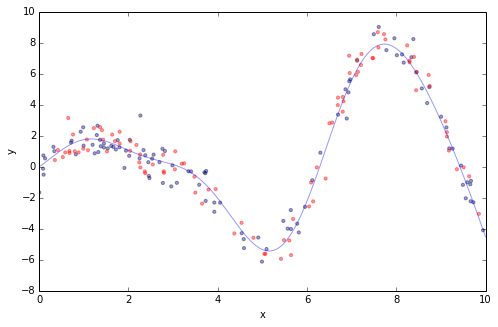
Gradient Boosting實戰 大多數的GBRT的應用效果可以用一條簡单的擬合曲線來展示,如下圖中用一個只有一個特徵x和相應變量y的回歸問題來舉例。我們隨機從數據集中均匀抽取100個訓練數據,用ground truth (sinoid函數; 淡藍色線) 擬合,加入一些隨機噪音。100個訓練數據之外(藍色),再用100個測試數據(紅色)來評估模型的效果。
1
2
3
4
5
6
7
8
9
10
11
12
13
14
15
16
17
18
19
20
21
22
23
24
25
26
27
28
29
30
31
32
33
34
import numpy as npdef ground_truth (x) : """Ground truth -- function to approximate""" return x * np.sin(x) + np.sin(2 * x) def gen_data (n_samples=200 ) : """generate training and testing data""" np.random.seed(13 ) x = np.random.uniform(0 , 10 , size=n_samples) x.sort() y = ground_truth(x) + 0.75 * np.random.normal(size=n_samples) train_mask = np.random.randint(0 , 2 , size=n_samples).astype(np.bool) x_train, y_train = x[train_mask, np.newaxis], y[train_mask] x_test, y_test = x[~train_mask, np.newaxis], y[~train_mask] return x_train, x_test, y_train, y_test X_train, X_test, y_train, y_test = gen_data(200 ) x_plot = np.linspace(0 , 10 , 500 ) def plot_data (figsize=(8 , 5 ) ) : fig = plt.figure(figsize=figsize) gt = plt.plot(x_plot, ground_truth(x_plot), alpha=0.4 , label='ground truth' ) plt.scatter(X_train, y_train, s=10 , alpha=0.4 ) plt.scatter(X_test, y_test, s=10 , alpha=0.4 , color='red' ) plt.xlim((0 , 10 )) plt.ylabel('y' ) plt.xlabel('x' ) plot_data(figsize=(8 , 5 ))
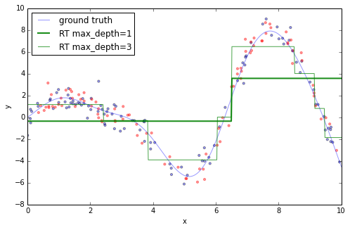
如果對以上數據僅使用一棵獨立的回歸樹,就只能得到區域内穩定的近似。數的深度越深,數據分割的越細緻,那麼能够解决的差異就越多。如下所示:
1
2
3
4
5
6
7
8
9
10
11
12
13
from sklearn.tree import DecisionTreeRegressorplot_data() est = DecisionTreeRegressor(max_depth =1).fit(X_train, y_train) plt.plot(x_plot, est.predict(x_plot[:, np.newaxis]), label ='RT max_depth=1' , color ='g' , alpha =0.9, linewidth =2) est = DecisionTreeRegressor(max_depth =3).fit(X_train, y_train) plt.plot(x_plot, est.predict(x_plot[:, np.newaxis]), label ='RT max_depth=3' , color ='g' , alpha =0.7, linewidth =1) plt.legend(loc ='upper left' ) Out[6]: <matplotlib.legend.Legend at 0x5706590>
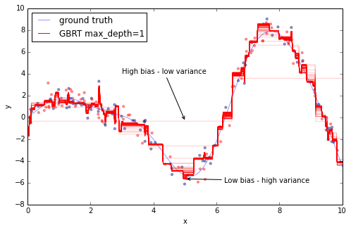
接下來,我們可以使用gradient boosting模型來擬合訓練數據,然後看著随著添加更多的樹,預測值與實際值的近似度是如何提升的。Scikit-learn的gradient boosting Estimator可以通過staged_(predict|predict_proba) 方法,評估模型預測效果,该方法返回一個生成器可以随著添加越来越多的树,迭代評估預測結果。
1
2
3
4
5
6
7
8
9
10
11
12
13
14
15
16
17
18
19
20
21
22
23
24
25
26
27
28
29
from itertools import islice plot_data() est = GradientBoostingRegressor(n_estimators=1000, max_depth=1, learning_rate=1.0) est.fit(X_train, y_train) ax = plt.gca()first = Truefor pred in islice(est.staged_predict(x_plot[:, np.newaxis]), 0 , 1000 , 10 ): plt.plot(x_plot, pred, color='r', alpha=0.2) if first: ax.annotate('High bias - low variance', xy=(x_plot[x_plot.shape[0] // 2 ], pred[x_plot.shape[0 ] // 2 ]), xycoords='data', xytext=(3, 4 ), textcoords='data', arrowprops=dict(arrowstyle="->", connectionstyle="arc")) first = False pred = est.predict(x_plot[:, np.newaxis])plt.plot(x_plot, pred, color='r', label='GBRT max_depth=1') ax.annotate('Low bias - high variance', xy=(x_plot[x_plot.shape[0] // 2 ], pred[x_plot.shape[0 ] // 2 ]), xycoords='data', xytext=(6.25, -6 ), textcoords='data', arrowprops=dict(arrowstyle="->", connectionstyle="arc")) plt.legend(loc='upper left') Out[7 ]: <matplotlib.legend.Legend at 0 x5d72f10>
上圖中50條紅線,每條代表GBRT模型增加20棵樹後的效果。可以看到,剛开始預測近似度非常粗,但随著添加更多的樹,模型可以覆盖到更多的偏差,最終產生紧密的紅線。
可以看到,向GBRT添加的更多的樹以及更深的深度,可以捕获更多的偏差,因此我們模型也更複雜。但和以往一樣,機器學習模型的複雜度是以“过擬合”為代價的。
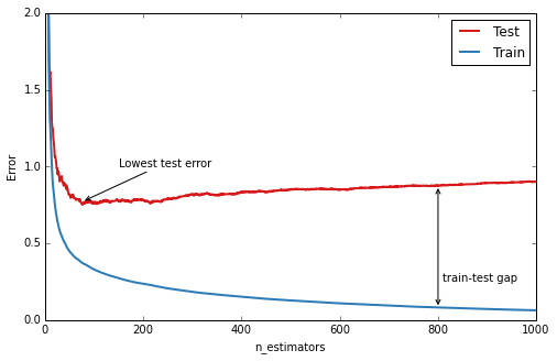
GBRT實戰中重要的診斷方法是使用異常座標圖來展示訓練集/測試集的錯誤(或異常),以樹的數量為横座標。
1
2
3
4
5
6
7
8
9
10
11
12
13
14
15
16
17
18
19
20
21
22
23
24
25
26
27
28
29
30
31
32
33
34
35
36
37
38
n_estimators = len(est.estimators_) def deviance_plot (est, X_test, y_test, ax=None, label='' , train_color='#2c7bb6' , test_color='#d7191c' , alpha=1.0 ) : """Deviance plot for ``est``, use ``X_test`` and ``y_test`` for test error. """ test_dev = np.empty(n_estimators) for i, pred in enumerate(est.staged_predict(X_test)): test_dev[i] = est.loss_(y_test, pred) if ax is None : fig = plt.figure(figsize=(8 , 5 )) ax = plt.gca() ax.plot(np.arange(n_estimators) + 1 , test_dev, color=test_color, label='Test %s' % label, linewidth=2 , alpha=alpha) ax.plot(np.arange(n_estimators) + 1 , est.train_score_, color=train_color, label='Train %s' % label, linewidth=2 , alpha=alpha) ax.set_ylabel('Error' ) ax.set_xlabel('n_estimators' ) ax.set_ylim((0 , 2 )) return test_dev, axtest_dev, ax = deviance_plot(est, X_test, y_test) ax.legend(loc='upper right' ) ax.annotate('Lowest test error' , xy=(test_dev.argmin() + 1 , test_dev.min() + 0.02 ), xycoords='data' , xytext=(150 , 1.0 ), textcoords='data' , arrowprops=dict(arrowstyle="->" , connectionstyle="arc" ), ) ann = ax.annotate('' , xy=(800 , test_dev[799 ]), xycoords='data' , xytext=(800 , est.train_score_[799 ]), textcoords='data' , arrowprops=dict(arrowstyle="<->" )) ax.text(810 , 0.25 , 'train-test gap' ) Out[8 ]: <matplotlib.text.Text at 0x5f10a90 >
上圖中藍線是指訓練集的預測偏差:可以看到開始階段快速下降,之後随著添加更多的樹而逐步降低。測試集預測偏差(紅線)同樣在開始階段快速下降,但是之後速度降低很快達到了最小值(50棵樹左右),之後甚至開始上升。這就是我们所指的“过擬合”:在一定階段,模型能够非常好的擬合訓練數據的特點(這個例子裡是我們隨機生成的噪音)但是對於新的未知數據其能力受到限制。圖中在訓練數據與測試數據的預測偏差中存在的巨大的差異,就是“过擬合”的一個信号。
Gradient boosting很棒的一點,是提供了一系列“把手”來控制過擬合,又被稱為“regularization”。
Regularization GBRT提供三個“把手”來控制“過擬合”:樹結構(tree structure),收斂(shrinkage), 隨機性(randomization)。
### 樹結構(tree structure)
單棵樹的深度是模型複雜度的一方面。樹的深度基本上控制了特征相互作用的成都。例如,如果想覆蓋維度特征和精度特征之間的交叉關系特征,需要深度至少為2的樹來覆蓋。不幸的是,特征相互作用的程度是預先未知的,但通常設置的比較低較好–實戰中,深度4-6常得到最佳結果。在scikit-learn中,可以通過max_depth參數來限制樹的深度。
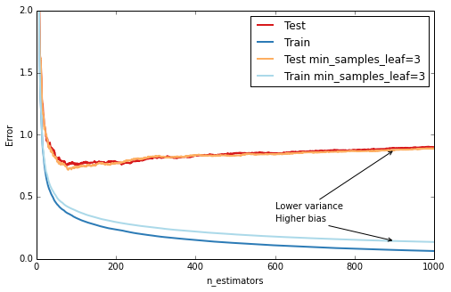
另一個控制樹的深度的方法是在葉節點的樣例數量上使用較低的邊界:這樣可以避免不均衡的劃分,出現一個葉節點僅有一個數據點構成。在scikit-learn中可以使用min_samples_leaf參數來實現。這是一個有效的方法來減少偏差,如下例所示:
1
2
3
4
5
6
7
8
9
10
11
12
13
14
15
16
17
18
19
20
21
22
23
24
25
26
def fmt_params(params): return ", " .join("{0}={1}" .format(key, val) for key, val in params.iteritems()) fig = plt.figure(figsize=(8, 5 ))ax = plt.gca()for params, (test_color, train_color) in [({}, (' ({'min_samples_leaf': 3 }, (' est = GradientBoostingRegressor(n_estimators=n_estimators, max_depth=1, learning_rate=1.0) est.set_params(**params) est.fit(X_train, y_train) test_dev, ax = deviance_plot(est, X_test, y_test, ax=ax, label=fmt_params(params), train_color=train_color, test_color=test_color) ax.annotate('Higher bias', xy=(900, est.train_score_[899 ]), xycoords='data', xytext=(600, 0.3 ), textcoords='data', arrowprops=dict(arrowstyle="->", connectionstyle="arc"), ) ax.annotate('Lower variance', xy=(900, test_dev[899 ]), xycoords='data', xytext=(600, 0.4 ), textcoords='data', arrowprops=dict(arrowstyle="->", connectionstyle="arc"), ) plt.legend(loc='upper right') Out[9 ]: <matplotlib.legend.Legend at 0 x5893a90>
### 收斂(Shrinkage)
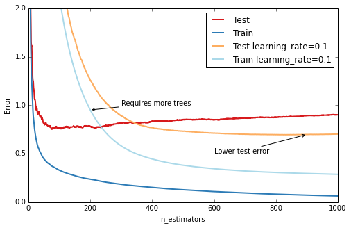
GBRT調參的技術最重要的就是收斂:基本想法是進行通過收斂每棵樹預測值進行緩慢學習,通過learning_rage來控制。較低的學習速率需要更高數量的n_estimators,以達到相同程度的訓練集誤差–用時間換準確度的。
1
2
3
4
5
6
7
8
9
10
11
12
13
14
15
16
17
18
19
20
21
22
23
fig = plt.figure(figsize=(8, 5 ))ax = plt.gca()for params, (test_color, train_color) in [({}, (' ({'learning_rate': 0.1 }, (' est = GradientBoostingRegressor(n_estimators=n_estimators, max_depth=1, learning_rate=1.0) est.set_params(**params) est.fit(X_train, y_train) test_dev, ax = deviance_plot(est, X_test, y_test, ax=ax, label=fmt_params(params), train_color=train_color, test_color=test_color) ax.annotate('Requires more trees', xy=(200, est.train_score_[199 ]), xycoords='data', xytext=(300, 1.0 ), textcoords='data', arrowprops=dict(arrowstyle="->", connectionstyle="arc"), ) ax.annotate('Lower test error', xy=(900, test_dev[899 ]), xycoords='data', xytext=(600, 0.5 ), textcoords='data', arrowprops=dict(arrowstyle="->", connectionstyle="arc"), ) plt.legend(loc='upper right') Out[10 ]: <matplotlib.legend.Legend at 0 x587b210>
### 隨機梯度推進(Stochastic Gradient Boosting)
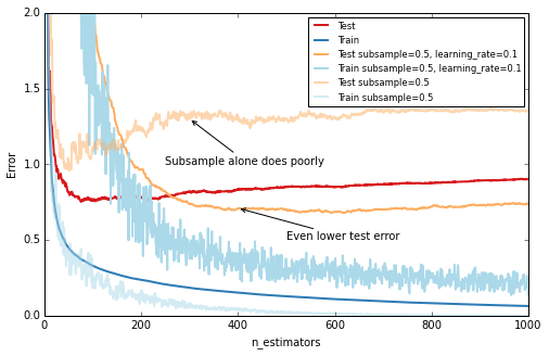
與隨機森林相似,在構建樹的過程中引入隨機性導致更高的準確率。Scikit-learn提供了兩種方法引入隨機性:a)在構建樹之前對訓練集進行隨機取樣(subsample);b)在找到最佳劃分節點前對所有特征取樣(max_features)。經驗表明,如果有充足的特征(大於30個)後者效果更佳。值得強調的是兩種選擇都會降低運算時間。
下文以subsample=0.5來展示效果,即使用50%的訓練集來訓練每棵樹:
1
2
3
4
5
6
7
8
9
10
11
12
13
14
15
16
17
18
19
20
21
22
23
24
25
26
27
28
29
fig = plt.figure(figsize=(8, 5 ))ax = plt.gca()for params, (test_color, train_color) in [({}, (' ({'learning_rate': 0.1 , 'subsample': 0.5 }, (' est = GradientBoostingRegressor(n_estimators=n_estimators, max_depth=1, learning_rate=1.0, random_state=1) est.set_params(**params) est.fit(X_train, y_train) test_dev, ax = deviance_plot(est, X_test, y_test, ax=ax, label=fmt_params(params), train_color=train_color, test_color=test_color) ax.annotate('Even lower test error', xy=(400, test_dev[399 ]), xycoords='data', xytext=(500, 0.5 ), textcoords='data', arrowprops=dict(arrowstyle="->", connectionstyle="arc"), ) est = GradientBoostingRegressor(n_estimators=n_estimators, max_depth=1, learning_rate=1.0, subsample=0.5) est.fit(X_train, y_train) test_dev, ax = deviance_plot(est, X_test, y_test, ax=ax, label=fmt_params({'subsample': 0.5 }), train_color='#abd9e9', test_color='#fdae61', alpha=0.5) ax.annotate('Subsample alone does poorly', xy=(300, test_dev[299 ]), xycoords='data', xytext=(250, 1.0 ), textcoords='data', arrowprops=dict(arrowstyle="->", connectionstyle="arc"), ) plt.legend(loc='upper right', fontsize='small') Out[11 ]: <matplotlib.legend.Legend at 0 x5889f10>
### 超參數調優(Hyperparameter tuning)
我們已經介紹了一系列參數,在機器學習中參數優化工作非常單調,尤其是參數之間相互影響,比如learning_rate和n_estimators, learning_rate和subsample, max_depth和max_features)。
對於gradient boosting模型我們通常使用以下“秘方”來優化參數:
1.根據要解決的問題選擇損失函數
2.n_estimators盡可能大(如3000)
3.通過grid search方法對max_depth, learning_rate, min_samples_leaf, 及max_features進行尋優
4.增加n_estimators,保持其它參數不變,再次對learning_rate調優
Scikit-learn提供了方便的API進行參數調優及grid search:
1
2
3
4
5
6
7
8
9
10
11
12
13
14
15
16
from sklearn.grid_search import GridSearchCVparam_grid = {'learning_rate' : [0.1 , 0.05 , 0.02 , 0.01 ], 'max_depth' : [4 , 6 ], 'min_samples_leaf' : [3 , 5 , 9 , 17 ], # 'max_features' : [1.0 , 0.3 , 0.1 ] ## not possible in our example (only 1 fx) } est = GradientBoostingRegressor(n_estimators=3000 ) # this may take some minutes gs_cv = GridSearchCV(est, param_grid, n_jobs=4 ).fit(X_train, y_train) # best hyperparameter setting gs_cv.best_params_ Out[12 ]: {'learning_rate' : 0.05 , 'max_depth' : 6 , 'min_samples_leaf' : 5 }
Origin